6-DOF serial robot kinematics

The task and the robots

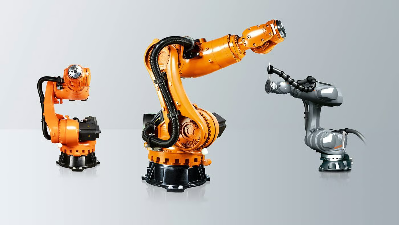
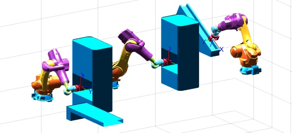
We proposed an industrial application and checked it could be done with industrial robots: a forging line for cast parts, based on a video of a real cell. Three KUKA KR 120 R2100 nano F exclusive robots, each with an on/off gripper, work in a row:

• Robot 1 picks a pre-mould from a plane inclined at 30° and puts it in the first press.
• Robot 2 takes the pressed part and loads it into the second press.
• Robot 3 takes the final part and drops it on a conveyor.

The study is purely kinematic: no dynamics, no control and no real robot. The goals were to avoid collisions with the machines, to avoid singular configurations and to keep speeds moderate and motions smooth. We worked in MATLAB with Peter Corke's Robotics Toolbox, a 3D robot model from the ARTE toolbox and a gripper we modelled ourselves.

Direct kinematics

From the robot dimensions in the datasheet we assigned the Denavit–Hartenberg frames and wrote the parameter table (d1 = 0.57 m, a1 = 0.30 m, a2 = 0.90 m, d4 = 0.90 m, d6 = 0.24 m, six revolute joints). In MATLAB it is a SerialLink object with the datasheet joint limits.

The three robots share the same DH matrix and differ in their base: robots 2 and 3 are translated and rotated to their place in the cell. The tool is a 0.2 m offset along z for the gripper. Our own function Transf_Sistemas_Total(R, q) multiplies the six link transforms and wraps the product with the base and the tool, which gives the pose of the gripper in the world frame.

Inverse kinematics

The wrist is spherical (the last three axes cross at one point), so we used Pieper's method, which splits the problem in two:

• Arm: the wrist centre is the tool position minus d6 along the tool z axis. From it come q1, q2 and q3 by geometry, with two arm configurations.
• Wrist: with q1 to q3 known, the remaining rotation (the transform from frame 3 to frame 6) gives q4, q5 and q6, with two wrist flips.

That gives up to eight solutions. CinInv(T, R, q0, best) first removes the base and the tool from the target pose and, if asked, returns the solution closest (smallest norm) to the previous posture, so the robot does not jump between configurations. The full derivation is in the report annex.

Velocities and singularities

The Jacobian is 6×6 and a symbolic analysis is unmanageable, so we looked for singularities numerically: we drew 10,000 random joint vectors in the workspace and kept those whose Jacobian determinant is zero.

Some patterns show up: q3 = −π/2 (links 2 and 3 align), q5 = 0 (links 3 and 5 align) and the joint limits. To check the first two, we forced q3 and then q5 to those values in all 10,000 random vectors, and every one of them came out singular. Other singular points have no simple relation between the joints.

These results then guided the trajectories: the waypoints and the inverse-kinematics solutions are chosen so the robots never go through those configurations.

Trajectory planning

Each robot has a short list of Cartesian waypoints (5 for robot 1, 7 for robot 2, 5 for robot 3): the pick and drop points plus intermediate positioning points. The drop point of one robot is the pick point of the next, so the three meet at the machines.

• Near a machine the robot enters and leaves slowly along a straight Cartesian line (ctraj). The inverse kinematics is solved on every sample and seeded with the previous posture, so the configuration does not jump along the segment.
• Away from the machines it interpolates in joint space, which gave cleaner and smoother motion than Cartesian interpolation between distant points.
• Joint interpolation uses mstraj on robot 1 and jtraj on robots 2 and 3: mstraj gave erratic speeds and large acceleration peaks, and avoiding them meant moving too slowly.
• For every waypoint we picked one of the eight inverse-kinematics solutions by hand when needed. On robot 1, for example, one point uses another solution so the wrist avoids q5 = 0.

Velocity and acceleration come from numerical differentiation with a step of 0.1 s.

Trajectory results

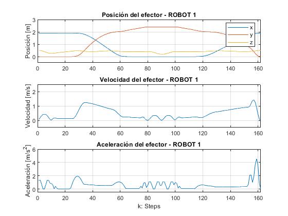
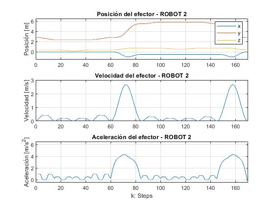
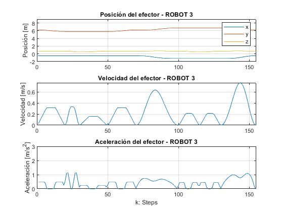
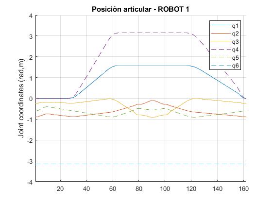
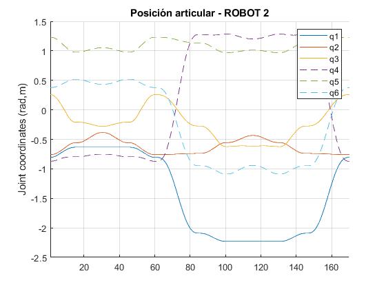
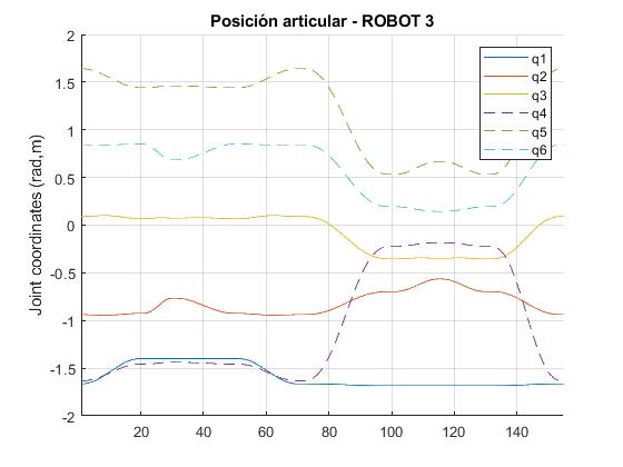
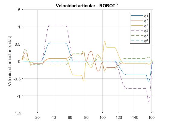
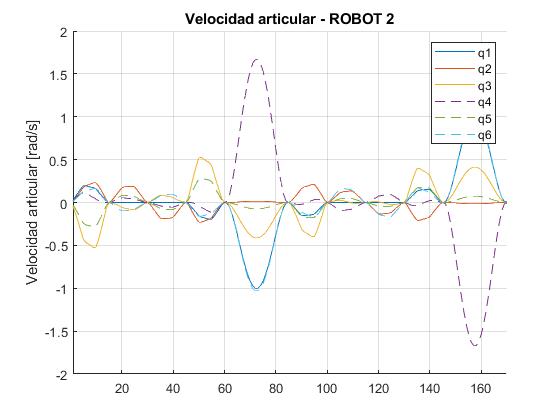
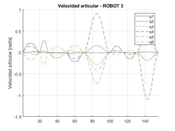
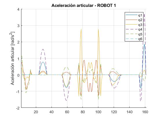
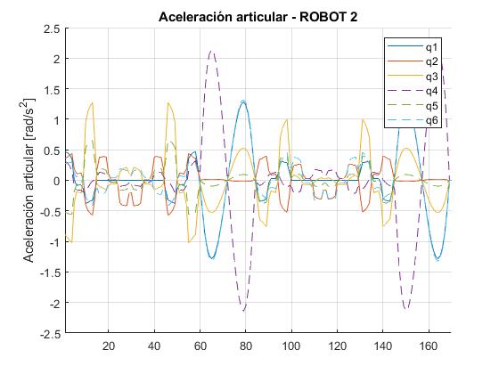
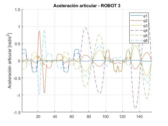
One column per robot; rows are the end-effector position, speed and acceleration, then joint position, joint velocity and joint acceleration. The horizontal axis is the step number (0.1 s per step).

The end-effector curves are smooth for the three robots. The only visible acceleration peak is at the end of robot 1's path, when it returns to the pick-up pose; it is small and that motion is not critical, so we accepted it. In robot 2 the largest joint speed is in the wrist joint q4, about 1.7 rad/s, during the long free moves.

Sensors and actuators (assumed)

The free datasheet does not say which sensors and actuators the robot has, so the report proposes what the task would need:

• Actuators: electric servomotors with their drivers, encoders for joint position and a mechanical holding brake on each.
• Current sensors, because they are simple and cheap. Motor temperature is inferred from the current (Joule heating), so there is no temperature sensor.
• Ultrasonic proximity sensors on the gripper and the arm to keep a minimum distance from objects and people (for example a Siemens 3RG6013-3AD00, 200–1300 mm).
• No force sensor: the parts are standardised, so the grip force is set in advance.

Limits

• Everything is kinematic. There is no dynamics, no control and no check of torques or real speed limits.
• Collision avoidance is not computed: we placed the waypoints by hand and checked the clearance visually in the 3D animation.
• Singularity avoidance is manual too (waypoints and the choice of inverse-kinematics solution), not an automatic planner.
• Each robot's trajectory is generated and animated on its own; nothing schedules the hand-offs between robots.
• Validation is visual and qualitative: the animation and the smoothness of the curves.