PMSM vector control design

The problem and the plan

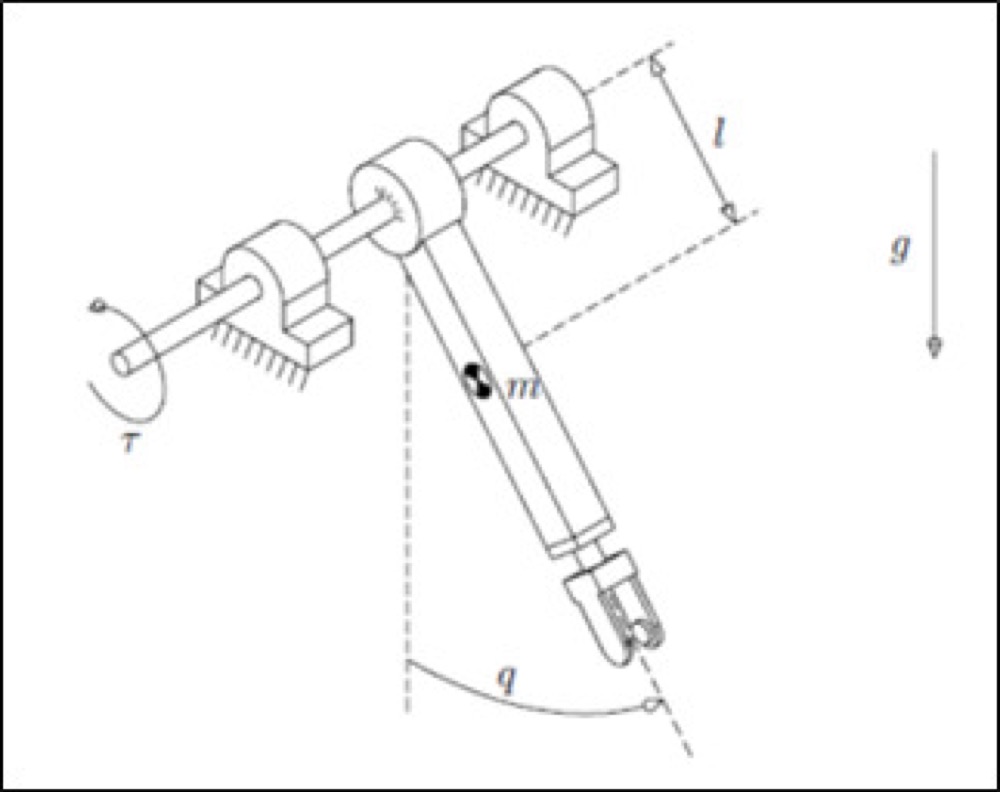
The goal is to control the position of the horizontal axis of one joint of an elementary robot arm. The joint behaves as a rigid pendulum under gravity, driven by a three-phase permanent-magnet synchronous motor (PMSM) fed by a three-phase inverter, through a 120:1 planetary gearbox. It has an encoder on the motor shaft, three phase-current sensors and a stator temperature sensor, and the payload at the end of the arm can go up to 1.5 kg. Everything is done in simulation with MATLAB/Simulink; there is no hardware.

We followed this order:

• Model the physics: mechanics, electromagnetics and heat.
• Linearise the model and analyse stability, observability and controllability.
• Simulate the open loop and find the operating limits of the motor.
• Design the controller: torque modulator, PID motion loop and observer.
• Verify against the real component limits and fix what fails.
• Replace the ideal sensors and inverter with realistic ones.
• Discretise the controller and program it as code.

Physical model

We built the plant in Simulink from three coupled subsystems:

• Mechanics: the pendulum with its gravity torque and a variable payload, the gearbox, and the rotor, all referred to the rotor shaft as a single equivalent inertia and friction.
• Electromagnetics: a salient-pole PMSM (Ld different from Lq) written in rotating qd0 axes through the Park transform. In these axes the torque depends on the q and d currents, and the three phase quantities become two.
• Heat: a first-order stator model with copper (Joule) losses, where the stator resistance grows with temperature.

At this stage the inverter and the sensors are ideal (unit gain). The component limits come from the course guide: gearbox output of 17 Nm continuous and 45 Nm peak, stator current of 0.57 A continuous and 2.83 A peak, and an inverter of up to 48 V line voltage (the motor accepts 30 V).

Linearisation and analysis

The plant is nonlinear, so we derived linear versions to design with:

• Jacobian linearisation around a slowly varying operating point, which gives an LPV model (an LTI one if the point is fixed).
• Nonlinear feedback linearisation: forcing the d-axis current to zero and treating the temperature as slow makes the motor behave like a separately excited DC machine. We call it the augmented LTI model.

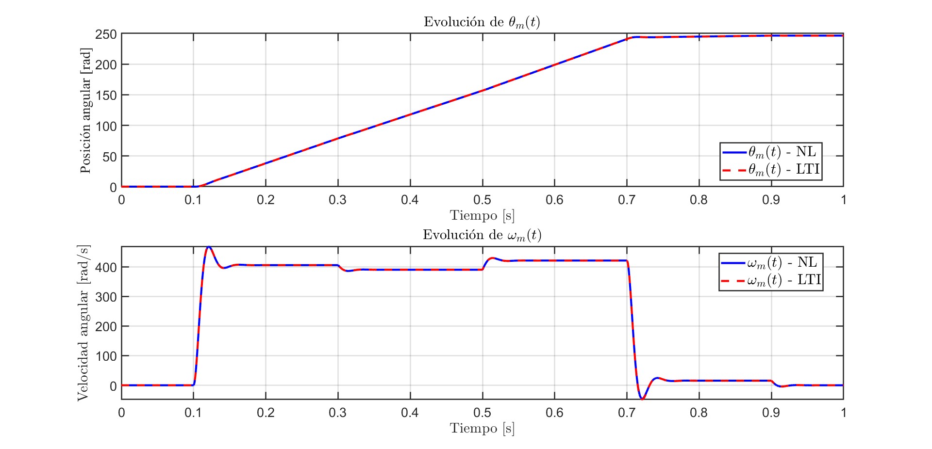
In open loop the two models are practically identical. The system is stable and underdamped: more payload lowers the natural frequency and raises the damping, and higher temperature moves the poles further left. Kalman tests say it is controllable and observable from the position measurement, but not from the speed alone, which is why the controller needs the position sensor to estimate speed.

Open-loop simulations and motor limits

We excited the nonlinear model with a voltage pulse and a double load-torque pulse and checked the internal states: speed, currents, voltages and temperature. A voltage pulse on the d axis showed the field strengthening and weakening effects: it changes the torque peaks and the voltages the inverter has to supply.

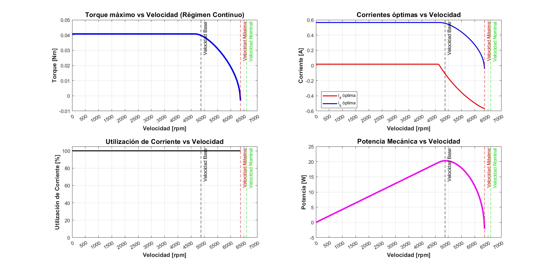
With the current and voltage limits we then drew the motor envelope. The maximum torque is about 0.041 N·m up to a base speed of about 4790 rpm. Beyond that the d current must go negative (field weakening) so the voltage does not saturate, and the torque falls until the speed limit of about 6370 rpm, below the 6600 rpm nominal. The maximum mechanical power is about 20 W. Another finding: for payloads above 0.5 kg the gravity torque at the motor exceeds what the continuous current limit allows, so covering the whole payload range would need a larger reduction ratio or a stronger motor.

Controller design

A cascade with a fast inner loop for current and torque and a slower outer loop for position and speed:

• Torque modulator (inner). First it cancels the motor's natural feedbacks, so each current derivative depends directly on one virtual voltage. We checked that this only works if the stator resistance follows its temperature: with a fixed resistance the proportionality is lost. Then a proportional current loop per axis, which acts as a virtual resistance, puts the poles at −5000 rad/s (about 800 Hz). Finally the torque reference is turned into a q current, compensating viscous friction and the gravity torque by nonlinear feedback. The d current reference stays at zero unless we want field weakening.
• Motion loop (outer): a PID that turns position and speed errors into a torque reference. We placed its poles with a desired polynomial (damping 0.75, natural frequency 800 rad/s) using the nominal inertia, and checked how they move with the payload: a heavier arm is slower but always stable. The integral action gives zero steady-state error and fully rejects a constant load.
• Observer: a reduced-order observer estimates position and speed from the encoder, with poles at −3200 rad/s. Under a constant load torque it left a steady error, so we added an integral term that also estimates the load torque. It follows constant loads exactly but not sinusoidal ones, which would need an internal model.

A few Python scripts reproduce the pole maps and compute the PID gains.

Checking the limits: the motion profile

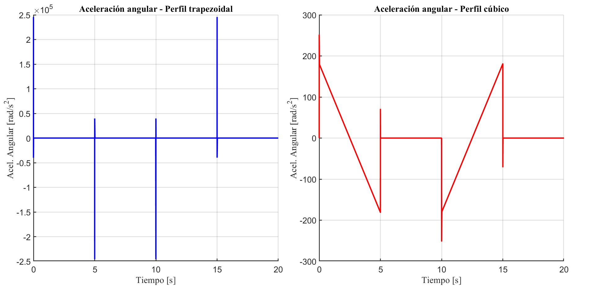
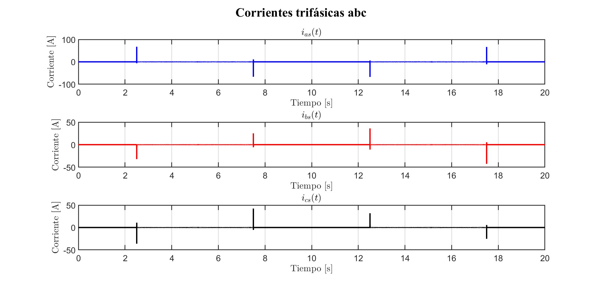
We first drove the joint with a trapezoidal position profile. It tracked well, but the abrupt changes of slope create speed steps, and the check against the component limits failed badly: the acceleration spikes reached about 2.5×10⁵ rad/s², the stator current peaked at about 66 A against 2.83 A allowed, the phase voltage at about 2300 V against 24 V, the gearbox torque at about 170 N·m against 45 N·m, and the stator heated up at every peak.

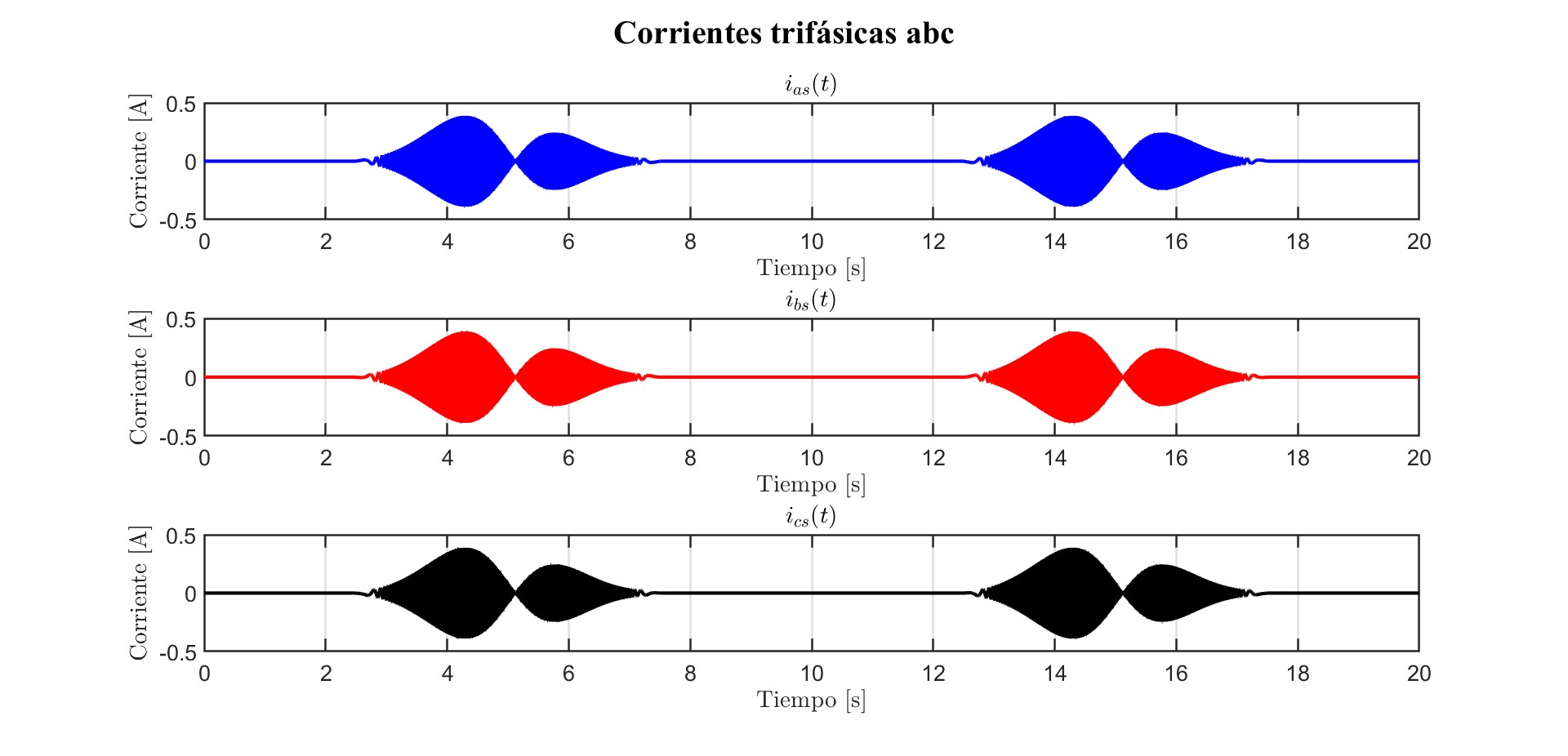
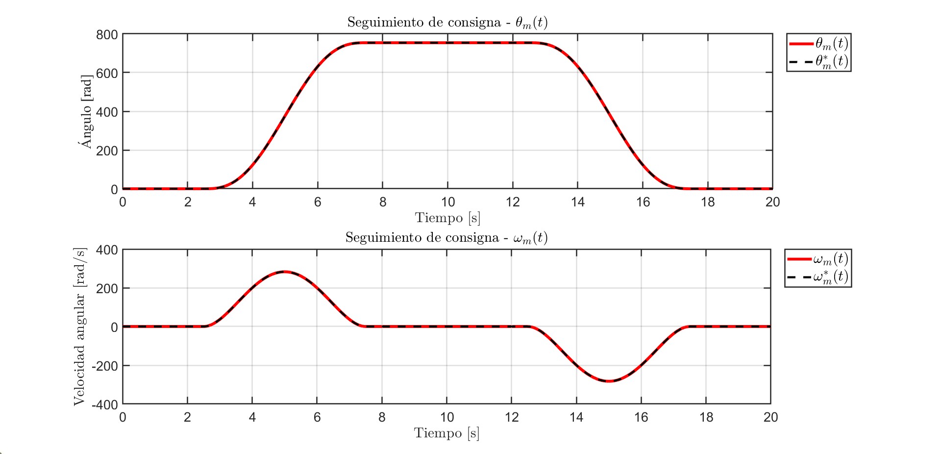
Instead of detuning the controller we changed the reference. A fifth-degree polynomial profile (rest to rest, 5 s per move, one full turn and back) rounds the corners in position and speed. The acceleration peaks drop to about 250 rad/s², the currents stay below 0.5 A, the voltages around 14 V, the gearbox torque is within its limits and the stator barely warms up.

Thermal check

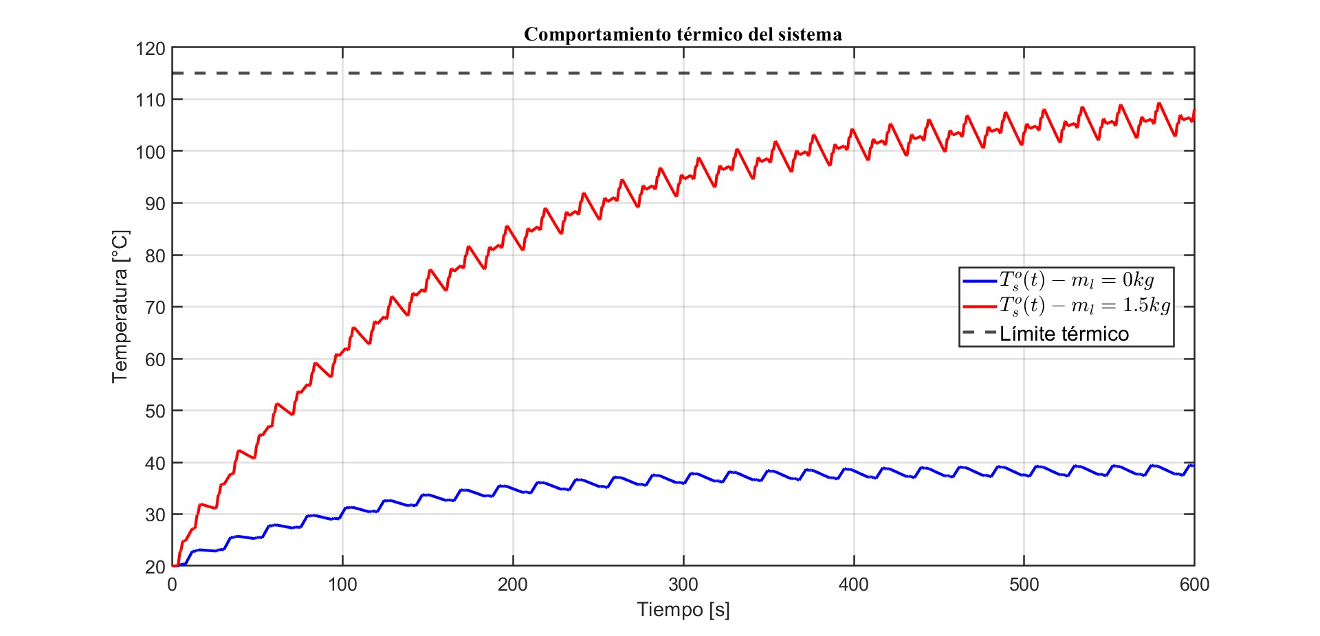
We repeated the motion cycle continuously (20 s per cycle, with a 5 N·m load-torque step between 8 s and 12 s) with no payload and with the maximum one, and watched the stator temperature. At 20 °C ambient both stay under the thermal limit, but with 1.5 kg the temperature climbs close to it, so a higher ambient would cross it. The maximum payload that can be carried cyclically without crossing the limit is 1.5 kg at 20 °C, 1.45 kg at 25 °C, 1.4 kg at 30 °C, 1.3 kg at 35 °C and 1.2 kg at 40 °C. In a real installation this would call for cooling or ventilation.

Non-ideal sensors and inverter

Up to here sensors and inverter were perfect. We modelled them as low-pass filters (second order for the position and current sensors and for the voltage modulator, first order for the temperature sensor), and added saturation to the modulator at its voltage limits.

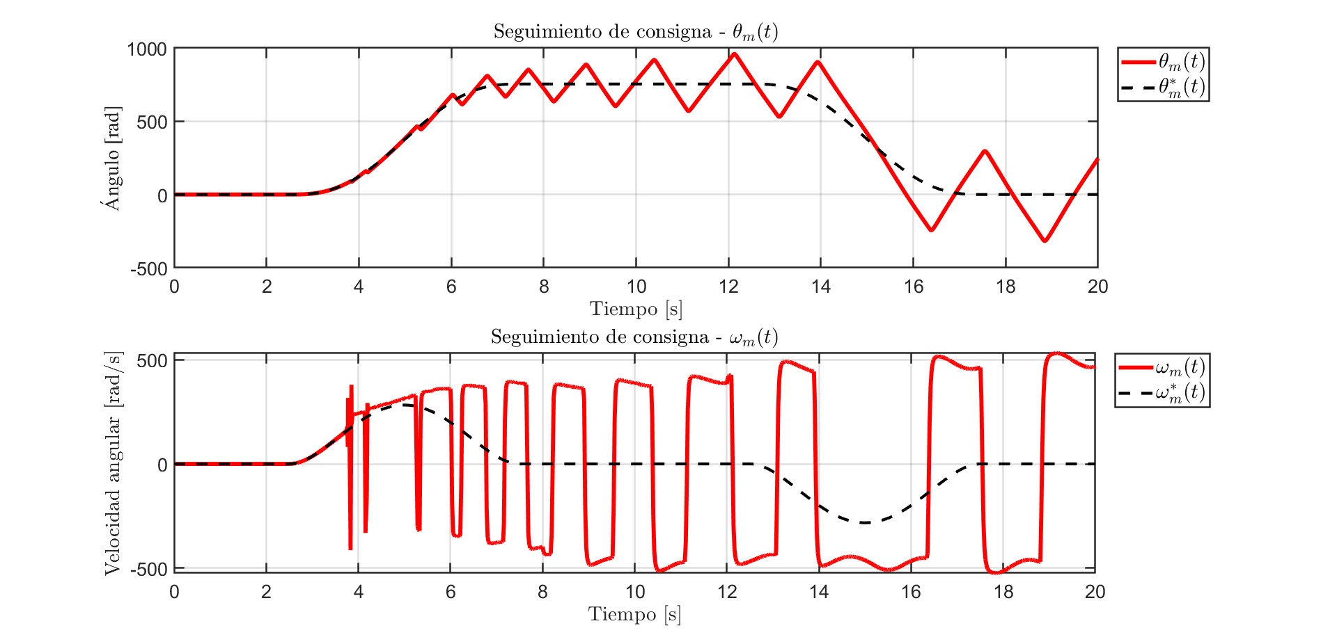
With slow components the system broke. With the first sensor parameters the simulation diverged after 0.03 s, and with a slow voltage modulator the system could not follow the references: the modulator ran saturated and the controller asked for impossible voltages. Raising the modulator bandwidth to 7000 rad/s fixed it. When everything non-ideal was active at once we had to raise them further: position sensor 12000 rad/s, current sensor 20000 rad/s and voltage modulator 24000 rad/s, with a 1 s temperature sensor. The lesson is that an inner loop at 5000 rad/s needs much faster sensors and inverter, and the report turns this into minimum specifications for the real components.

Discretisation and programmed controller

To get closer to a real implementation we discretised the controller with Tustin's method, which turns every integrator into a trapezoidal sum. The sample time comes from the fastest loop, the current loop at 5000 rad/s (about 800 Hz): the 10 to 20 times rule gives a minimum of about 84 µs, and we used 10 µs. Zero-order holds were added to the sensor signals and to the controller outputs. The tracking, the limits and the temperature stay as good as before, and zooming in on the measured position shows the steps from sampling.

Then we replaced all the controller block diagrams with one MATLAB function block that holds the whole controller: observer, PID with anti-windup, torque modulator, current loops, decoupling and inverse Park transform, with the state kept between calls. The curves are the same as with the block diagram.

Results

The final system, with non-ideal sensors and inverter, a discretised controller and the fifth-degree profile, follows position and speed references and stays inside the voltage, current and torque limits of the components. In the disturbance test a 5 N·m load step is applied between 8 s and 12 s, with no payload and with 1.5 kg: the position deviation is almost imperceptible and the speed shows short oscillations. With ideal sensors, the observer's largest estimation errors are about 1.2×10⁻⁴ rad in position and 0.75 rad/s in speed.

Limits and next steps

• It is all simulation: there is no hardware, the inverter is an averaged model and the sensors are filters, so the real behaviour could differ.
• The drive cannot cover the full 0 to 1.5 kg payload range in continuous duty without exceeding the current limit, and at high ambient temperature the payload has to be reduced.
• The load-torque estimate is exact for constant loads but not for sinusoidal ones.
• Next: include the real dynamics of the chosen sensors and actuators from the first modelling stage, and test the programmed controller on a microcontroller with hardware-in-the-loop.